\(\chi\) parameters
\(\chi\) parameters introduced by Ackland and Jones measures the angles generated by pairs of neighbor atom around the host atom, and assigns it to a histogram to calculate a local structure. In this example, we will create different crystal structures and see how the \(\chi\) parameters change with respect to the local coordination.
[1]:
import pyscal.core as pc
import pyscal.crystal_structures as pcs
import matplotlib.pyplot as plt
import numpy as np
The :mod:~pyscal.crystal_structures module is used to create different perfect crystal structures. The created atoms and simulation box is then assigned to a :class:~pyscal.core.System object. For this example, fcc, bcc, hcp and diamond structures are created.
[2]:
fcc_atoms, fcc_box = pcs.make_crystal('fcc', lattice_constant=4, repetitions=[4,4,4])
fcc = pc.System()
fcc.atoms = fcc_atoms
fcc.box = fcc_box
[3]:
bcc_atoms, bcc_box = pcs.make_crystal('bcc', lattice_constant=4, repetitions=[4,4,4])
bcc = pc.System()
bcc.atoms = bcc_atoms
bcc.box = bcc_box
[4]:
hcp_atoms, hcp_box = pcs.make_crystal('hcp', lattice_constant=4, repetitions=[4,4,4])
hcp = pc.System()
hcp.atoms = hcp_atoms
hcp.box = hcp_box
[5]:
dia_atoms, dia_box = pcs.make_crystal('diamond', lattice_constant=4, repetitions=[4,4,4])
dia = pc.System()
dia.atoms = dia_atoms
dia.box = dia_box
Before calculating \(\chi\) parameters, the neighbors for each atom need to be found.
[6]:
fcc.find_neighbors(method='cutoff', cutoff='adaptive')
bcc.find_neighbors(method='cutoff', cutoff='adaptive')
hcp.find_neighbors(method='cutoff', cutoff='adaptive')
dia.find_neighbors(method='cutoff', cutoff='adaptive')
Now, \(\chi\) parameters can be calculated
[7]:
fcc.calculate_chiparams()
bcc.calculate_chiparams()
hcp.calculate_chiparams()
dia.calculate_chiparams()
The calculated parameters for each atom can be accessed using the :attr:~pyscal.catom.Atom.chiparams attribute.
[8]:
fcc_atoms = fcc.atoms
bcc_atoms = bcc.atoms
hcp_atoms = hcp.atoms
dia_atoms = dia.atoms
[9]:
fcc_atoms[10].chiparams
[9]:
[6, 0, 0, 0, 24, 12, 0, 24, 0]
The output is an array of length 9 which shows the number of neighbor angles found within specific bins as explained here. The output for one atom from each structure is shown below.
[28]:
plt.bar(np.array(range(9))-0.3, fcc_atoms[10].chiparams, width=0.2, label="fcc")
plt.bar(np.array(range(9))-0.1, bcc_atoms[10].chiparams, width=0.2, label="bcc")
plt.bar(np.array(range(9))+0.1, hcp_atoms[10].chiparams, width=0.2, label="hcp")
plt.bar(np.array(range(9))+0.3, dia_atoms[10].chiparams, width=0.2, label="diamond")
plt.xlabel("$\chi$")
plt.ylabel("Number of angles")
plt.legend()
[28]:
<matplotlib.legend.Legend at 0x7f2f4f408650>
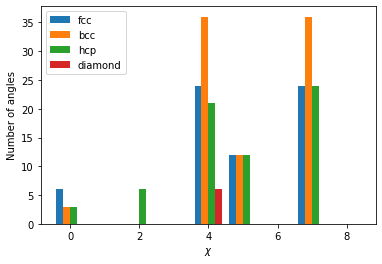
The atoms exhibit a distinct fingerprint for each structure. Structural identification can be made up comparing the ratio of various \(\chi\) parameters as described in the original publication.